AI systems seem to be amongst the most complex systems humankind has ever built, containing sets of interacting AI models, run across hundreds of computing chips which were produced on nanometre precision. However, while the systems seem complex, their underlying blueprint is surprisingly simple: let’s increase the maximum number of (mathematical) operations we can execute per second, and intelligence will follow. This blueprint was given to us by the Neural Language Model Scaling Laws that were a useful license to scale our systems homogeneously using a small set of algorithms and types of hardware, in the pure pursuit of FLOPs.

While such homogeneous system scaling has been consuming a whole lot of attention, we started seeing new patterns developing that fall outside the established scaling laws. This is not only our blog post about heterogeneous agents on heterogeneous hardware showing benchmark beating performance, but also that new kinds of heterogeneous temporal operations easily beat established ones or entirely new accelerator designs running new model architectures at efficiency impossible on established hardware. These suggest a fundamentally new blueprint, one that pursues heterogeneity first, and only pursues FLOPs where they can drive us towards that heterogeneity. Working out whether this is the direction to focus our attention on is quite literally a trillion dollar question, given the global spend on AI and compute infrastructure.

Spending a trillion dollars on a specific strategy ideally does not purely rely on a set of empirical observations of the type ‘the line goes up’, but uses systematic model-based estimations of how systems improve in their capabilities, while also doing so in a way that ends up with the realisation of the capabilities being economically viable. To provide these model-based estimations, we poured over more than 80 years of scientific evidence for how ideal systems scale as they strive to increase performance and efficiency and integrated them into what we call The Principle of Maximum Heterogeneity. This principle shows optimising towards heterogeneity is the natural optimisation strategy for solving any complex problem and that by doing so, one achieves performance, efficiency, and robustness, on the Pareto front unachievable by homogeneous solutions. We show that this performance and efficiency benefit of heterogeneity only ever increases with problem complexity and resource constraints, so that we will specifically need heterogeneity for the most complex problems we hope to solve with AI at scale.

Here we will walk through the process that it takes to derive The Principle of Maximum Heterogeneity to introduce not only the result, but also how we got there. A much more technical treatment with all derivations and definitions can be found in the accompanying full paper.

The question ‘how should we scale our AI and compute systems?’ is difficult to answer as we live in a time when what we want to achieve with these systems is changing day by day, as new capabilities come into reach, and goal posts are being moved, because our ideas of what technology can do expands and expands. Really what ought to underlie the answer to this question is an even more fundamental question: ‘how does any system, that solves the kind of problems we care about, scale?’. This is the way we can arrive at an answer that generalises as our goal posts for capabilities and the hardware parts we use in our systems change. An answer that derives from our fundamental understanding of how complex systems work.

The best way to answer this is to first define what kind of system an AI-compute system is: what entities it contains, how they interact, and how the system scales. Finding a representation that is both accurate and simple is key. Simple enough to generalise mathematically, but accurate enough to capture the system's real scaling behaviour. We define an AI-compute system as solving a task, described as a distribution of operations - reasoning, planning, searching, summarising, abstracting, and so on. These operations are jointly solved by a network of processing elements, which we call agents.

We define an agent as any entity that can transform its own skill density into a production density. An agentic system is an interaction network of n such agents, where the collective production function those interacting agents produce can exceed the sum of its parts: whereby the integral of production function can be greater than n agents. Whether that production function meets a given demand - a task, a workload, a series of operations, a problem to be solved - determines whether the system works well or not. When it does, what you have is effectively an algorithm: a set of agents that have transformed their collective skill densities into the right production function for the task at hand, via their own interaction network.

This framing lets us reason precisely about which configurations - how many agents, which skills, what interaction structure - solve which problems better. And it has a recursive property. The skills an agent draws on were themselves produced by other agents beneath it, each transforming their own skills into production that became the skill of the layer above. What we call "hardware" is really just the abstraction boundary: it names which layer of agents below produced the particular skill function that the agentic system above now operates with.

This means that three classical terms in computing - workload, algorithm, and hardware - all resolve into the same underlying abstraction: agents and agentic systems. It is agents all the way down.

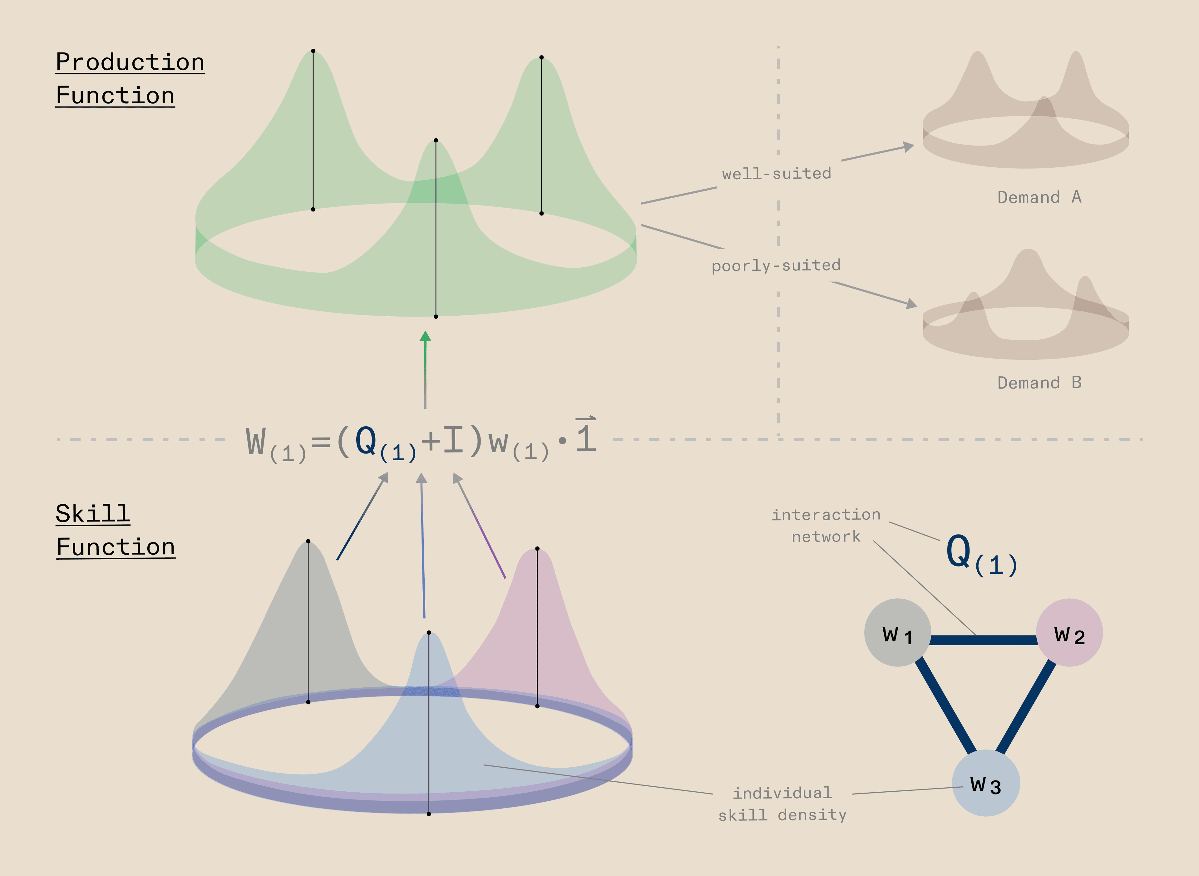
So how do we capture all the components we care about in a mathematical model? We represent the workload as a density over a 1D space, the cognitive operations space, where the dimension represents the kind of operation required and the density value at any given point represents the amount of that operation present in the workload. This distribution of the workload needs to be solved by underlying agents, themselves produced by hardware. Agents are Gaussian densities in a similar 1D space, the algorithm space, where the dimension represents the skills agents can have and the density value of a given agent represents how much of a particular skill it possesses, i.e., its talent for that skill.

To allow agents to collaborate and jointly produce a workload, they are connected to each other via network connections that we represent as a graph, where vertices are agents and edges are the communication connections between them. With this graph structure, the workload produced by the system is simply the communicability matrix of the graph multiplied by the vector of individual agent production functions. A workload is considered solved when the collaborating agents jointly cover the entire workload distribution.

Note that this works because in this simple formulation we assume the workload and the agents live in the same 1D space: for the workload, that space represents cognitive operations to be performed; for agents, it represents their algorithmic capacity for performing those operations. For the workload-layer to algorithm-layer, the operations might be cognitive in character, such as reasoning, searching, or summarising, whereas from algorithm-layer to hardware-layer these would be more computational in nature, such as memory load, mathematics, or iterative search. We model the hardware in exactly the same fashion as the network of agents above it, as Gaussian densities over their own space, jointly producing a workload across their own communication network. This gives the system an inherently hierarchical structure where each layer produces the one above it, which in its general form looks like:

or, written out for the specific three-layer system we have been discussing:

For simplicity we assume a direct linear mapping between layers here, but the full paper discusses how more complex mappings do generally not change the conclusions of our results.

Interestingly, the same composable structure also allows us to introduce constraints into the system in a natural way. Just as the hardware layer produces leftwards to meet the algorithm layer's demands, a constraint layer can be thought of as an additional production goal that the bottom layer must simultaneously satisfy, represented as a rightward arrow out of the bottom layer, meaning that layer must now produce in two directions at once:

This means that hardware limitations, energy budgets, or any other real-world constraint can be expressed in exactly the same mathematical language as the agents themselves, keeping the model clean and unified.

Finding the optimal systems-level architecture within this framework then takes naturally the form of a constrained optimisation problem. The objective is to find the agent skills and network topology that best meets the demand workload, given what the hardware layer can provide and whatever constraints are active. The cost function captures this as the minimal shortfall between what the system produces and what the workload demands,

where the indicator function ensures we only penalise the system for operations it fails to cover, as overshooting part of the workload is fine while undershooting is not. Using the p-norm keeps the cost function differentiable and amenable to standard gradient descent, allowing us to efficiently solve for the optimal agent composition across a wide range of configurations: different workload shapes, different numbers of agents, different numbers of layers, and different resource constraints.

Now that we have this relatively simple mathematical model of our system, we can use standard optimisation approaches with gradient descent to find what the best possible systems-level architecture is for different combinations of shapes of the workload, number of agents, levels of agents contained in the system, and any other constraints we can think of. What this allows us to do is to study how an optimal system would scale across a variety of parameters of the system, to study how any optimal system would behave in the limit, so in the future regime where any complex ability is solvable with our AI-compute systems. Some might call this AGI. We prefer to think of it in a way that AI-compute systems are distributed production systems, where agents come together across algorithms and hardware to jointly produce intelligence (or ‘information’ and ‘entropy reduction’, if you prefer it more formally). We can think of this as an information production as the property of many agents coming together during a joint production process can also be observed in other contexts, like economics and biology. What we want to discover is how any optimal distributed (AI-compute) production system should scale. However, before we can discover this ideal scaling, we need to validate that our model is correct about how complex systems behave.

Validating a model that ought to predict the best design for a system that (a) has never been built and (b) should produce capabilities not available today in any available system today, is inherently a difficult process, as the data for it does not yet exist. However, we are in luck, as of course we do have data on lots of systems, of the computing but also from other sectors that we can use.

To start with the validation data from AI and computing, we of course have the already discussed Neural Language Model Scaling Laws, or the newer iteration of it, in the form of the Chinchilla Scaling Laws. Those show that with increasing computational resources (FLOPs, model parameters, data) we achieve increasing task performance of the functional shape of a power-scaled reciprocal. So we can start there and see whether our model would predict this functional shape. To test this we assume a system that monotonically scales its compute resources of a predefined type and we also assume a workload with a multi-gaussian shape across the distribution of skills, which we ought to expect for any decently complex real world task. Under these assumptions our model does indeed show the typically observed scaling laws (Figure 2). Our model is off to a good start:

Now, however, we run into the typical problem of validating a model that explores new designs: many dimensions that the model could predict over are only very sparsely covered by the data, if at all. The existing scaling data does not at all speak to factors such as specialisation of agents, distribution of agents across skill space, or even just exact characteristics of skills the systems ought to solve a workload. They cover the dimension of the design space only very sparsely. Isolated small scale data does exist pointing towards increased robustness under data distribution shifts and increased learning abilities in AI-compute systems with more varied components. However, generally speaking those are only captured in very small scale systems that do not address the complex workloads we most care about. While we discuss how those are also explained by our model in the accompanying paper, we must think a bit out of the box to validate our model further with other large scale data.

In the same way that ‘history never repeats itself but it rhymes’, we have seen many times that the same underlying laws are at play across large scale systems, regardless of whether we are looking at biology, economics, or an artificial system. In fact, the very idea of scaling laws that took over our imagination in the context of AI-compute systems, has been discussed before in many other contexts of the natural environment. To be specific, our claim is that the fundamental principles that would optimise the scaling of AI-compute systems are not all that different from any other system where sets of imperfectly connected agents jointly coordinate (through collaboration or competition) to produce a joint output. As long as we believe that to be true, we can use data from any of these other systems to validate our model. Note that we are not claiming that AI-compute systems work exactly in the same way that the systems that we compare them to next, we just claim that the fundamental interactions that drive the scaling behaviour of these systems are the same.

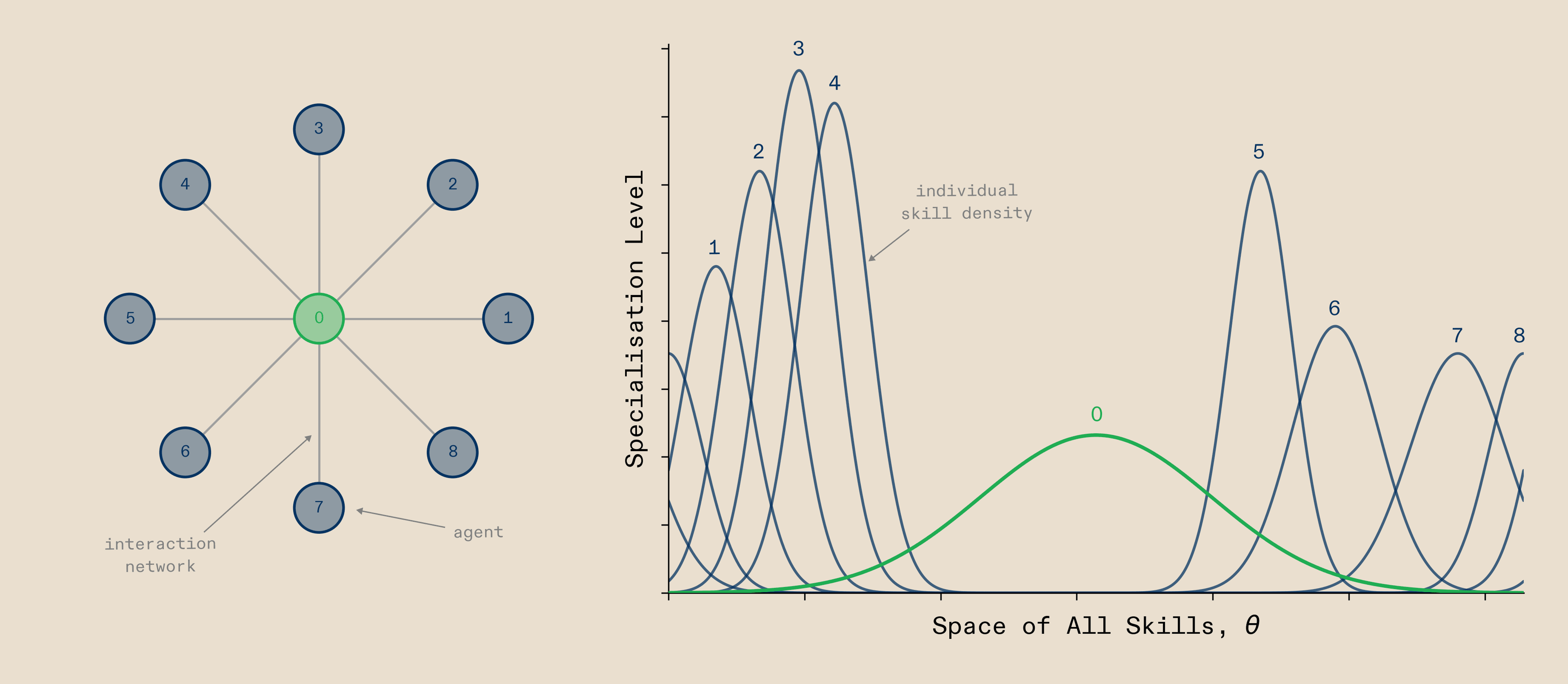
A natural comparison for AI-compute systems is the human/primate brain. It already solves the complex problems we care about and it is made of lots of regions that are imperfectly connected to jointly produce cognition. Hence we will use it as a first comparison point, starting with its macro-scale architecture, so the overall topology and connectivity of regions. What we observe in the brain is that when a complex task is solved, a large network of regions activates, with a generalist ‘Multiple-demand network’ region lying in the center position of the overall network of regions and more specialised regions connected to it in the periphery. Jointly they produce the cognition underlying intelligent behaviour. Interestingly our model predicts the same layout, as shown in Figure 3. When agents are arranged in a star-like topology during problem solving, they converge on putting the generalist network in the centre, with more specialised agents surrounding it. While this is data from the macro-scale / multi-region level, the investigations in the paper also show that our model can replicate the exact way that the neurons in these regions acquire their properties. While this is validating that our model captures how multiple regions / agents ideally collaborate during problem solving, we understand that ‘building compute systems like the brain’ is a bit of an outdated meme. So what if we looked at a very different and more manmade system?

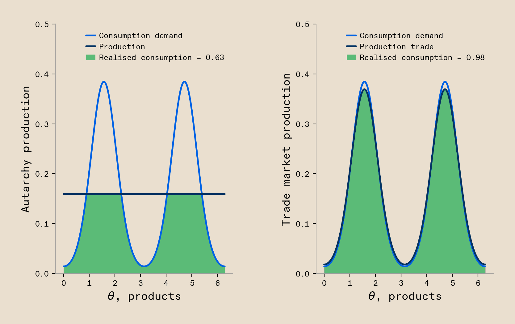
World-wide trade and dynamics in labour markets are another example where many agents produce a joint output through their interactions. We can observe a very well established case of this in the production and flow of goods in global trade. Leaving aside any considerations of sovereignty and instead focus on pure optimisation for productivity, as is the focus of our model, we observe that as countries start forming networks of collaborating regions, the optimal solution is increasingly to specialise, as each individual country’s possible productivity and welfare is higher when they specialise in producing a certain set of goods and trade to acquire the not-produced goods. Our model shows this, as countries, once connected through a (trade) network, start to specialise which allows them to maximise their overall welfare in return (Figure 4). We can observe another example of economic optimisation in the context of labour markets. Here we observe that in countries where the labour market is efficient, meaning that through good information flow and good worker-to-employer matching workers tend to find suitable employers, that workers tend more towards specialising. On the contrary, environments with worse labour markets incentives workers to stay generalists, with negative effects on the overall productivity of the economy. Again, our model can easily capture this data. When we allow for better communication between agents, the ideal solution shows more specialists than when we have poor communication (detailed modelling shown in paper).

We could go on. The full paper has many more examples of such systems, including a more technical description of what all these systems have in common so that a very simple mathematical model can capture so many nuances about their behavior, covering additional case studies in ecology, financial systems, and neuroscience, alongside more examples from computing. The fact that we can do this in itself is a mesmerising fact. It is worth pausing very briefly to appreciate that this simple model really captures something about how such distributed production systems work. Of course the reason we built the model was to validate the interactions in the system, so that we can then extrapolate its optimal scaling behaviour. So that is what we ought to do next.

Understanding why a model works the way it works can be much harder than building the model itself. Generally, when modelling complex systems we face the problem that if the model is too simple we cannot replicate any of the data from the systems we care about. On the flipside, if it is too complex, we end up struggling to extract the principles that drive the model’s behaviour. Our model promises to strike a good balance, as it generally relies on very simple mathematical relationships, but has already proven to capture systems-level data.

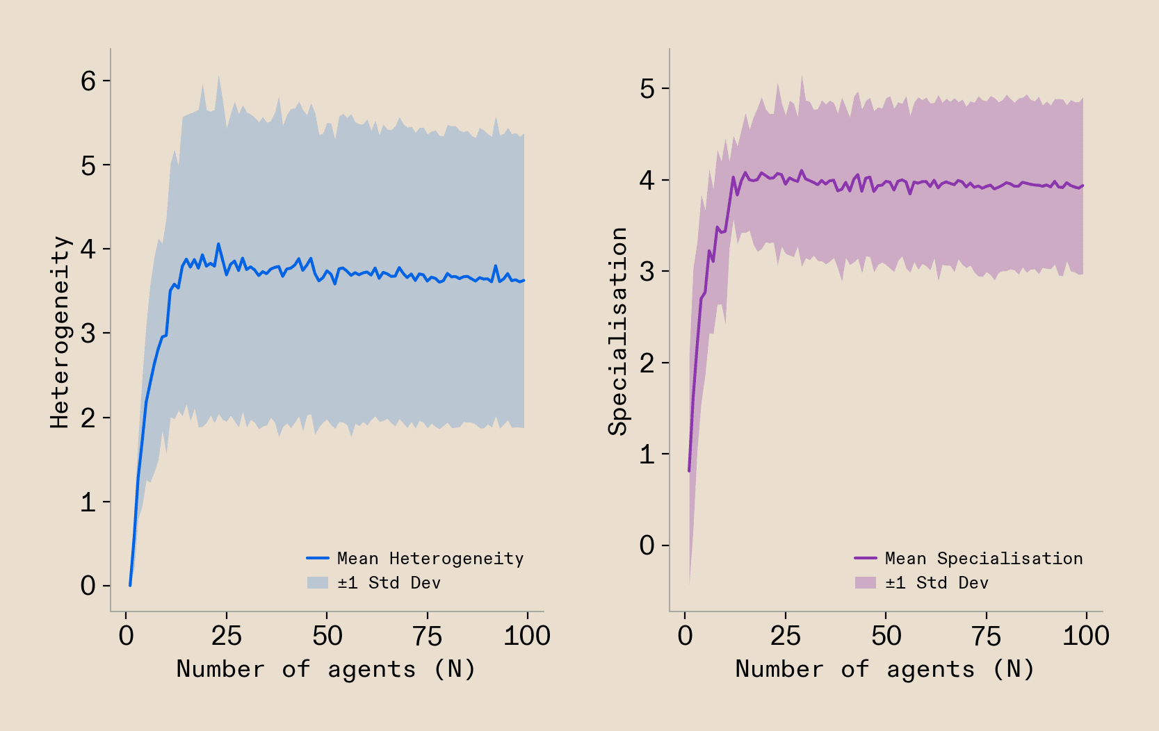
The question that got us into this model building to begin with was about the scaling behaviour of the model, so we will study this first. To do so, we will study how the ideal set of agents looks for solving complex tasks, as we scale up the number of agents that collaborate on the task solution. We study the degree of specialisation of all agents, the heterogeneity of the set of agents, and a range of other metrics that describe the ideal solution agents converge on. As of course the exact shape of the workload distribution will have some influence on that ideal solution, we run our analyses across a set of 16 different possible workload shapes and leave the question of the exact influence of the workload shape for later. Running this analysis, we observe a striking pattern when extracting the optimal agent composition over the size of the system measured in the number of agents: we see that agents rapidly increase the heterogeneity of their overall solution, alongside the average specialisation of all agents (Figure 5). Their first and most important optimisation objective clearly is to pursue systems-level heterogeneity.

We can now come back to the shape of the workloads and see how the optimisation drive towards heterogeneity is influenced by the shape of the workload. We can do so by measuring characteristics of the workload distribution and see how predictive they are of the drive towards heterogeneity. We find that the maximum spread of the workload, so the difference between the two most different operations that are present in the workload to a significant degree, is most predictive of the ideal level of heterogeneity of the solution. A higher spread of the workload causes more heterogeneity. Additional relationships like this can also be identified for specialisation, where non-uniform workloads are predictive of specialisation.

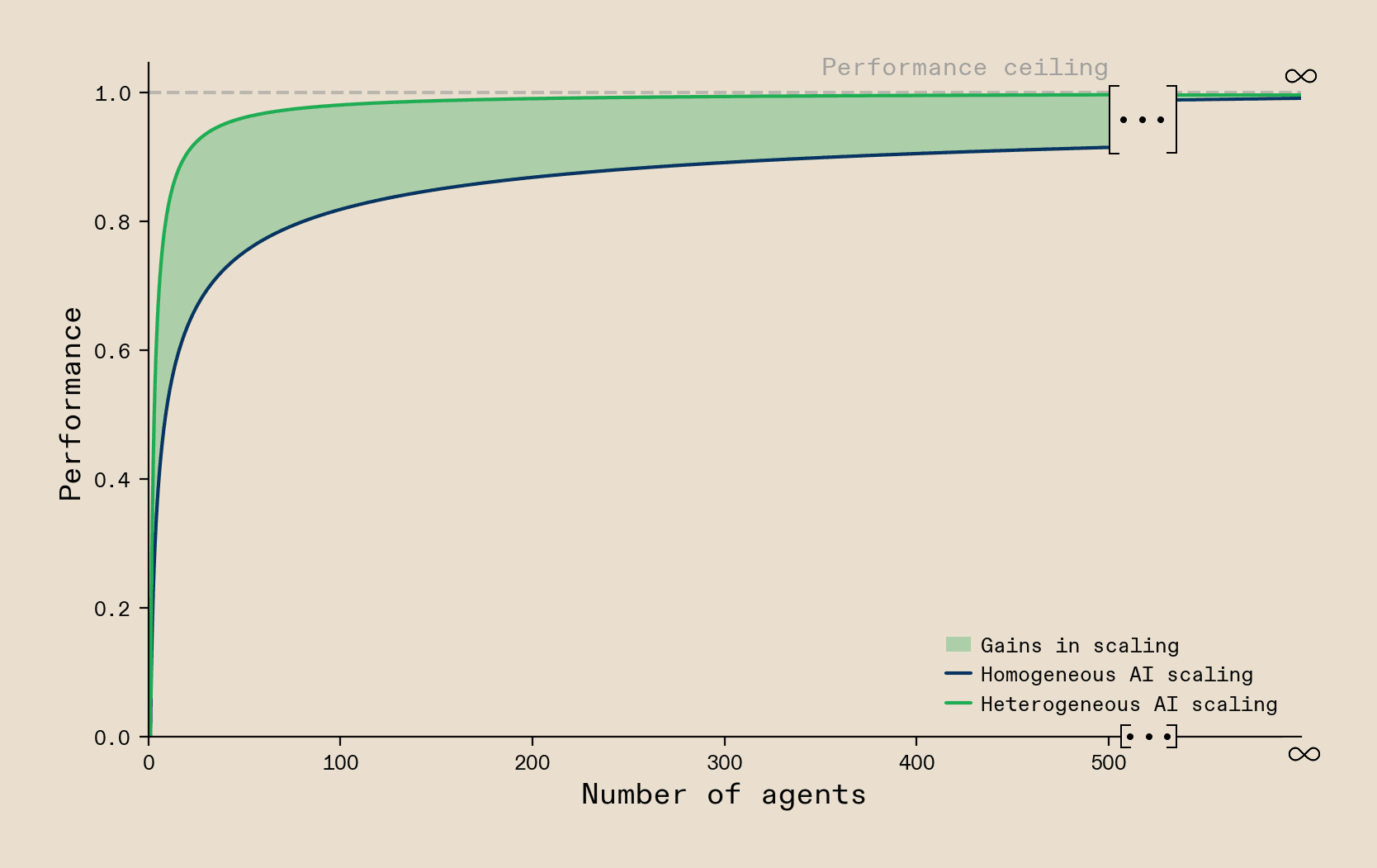
Our model also uncovers a property of system scaling that links heterogeneity to the efficiency and robustness of the system. Specifically, we find that once you add any resource constraints to the systems, so that you do not have unlimited compute resources or not an unlimited number of agents you can run, heterogeneous systems always dominate homogeneous solutions. This is because heterogeneous systems lie on a Pareto front across efficiency and robustness that is not achievable by any homogeneous solution (Figure 6). This finding strongly resonates with the Zeitgeist discussed in the community of researchers building AI-compute systems, which is that with unlimited resources you can just scale to infinity to achieve AGI. However, in any scenario where you need to do so with realistic constraints and perhaps even the goal of deploying the system at cost, you will naturally converge on a heterogeneous solution.

We summarise the set of findings around this pursuit of heterogeneity in, what we call, The Principle of Maximum Heterogeneity. The Principle of Maximum Heterogeneity has many additional interesting nuances that we lay out in the paper. Here we want to highlight one particularly striking one: the drive towards heterogeneity in systems is recursive! That means that if you have a system that is made of multiple layers – for example in the context of AI-compute systems we discussed workloads being at the top, followed by an algorithm layer, followed by a compute hardware layer – then the drive towards heterogeneity permeates across all layers of the system. The result of this is that all layers of the system drive towards heterogeneity as a function of the maximum spread of the workload distribution at the very top. There is no point where we can say ‘heterogeneity has been achieved on the top layer, we can now build an ideal system homogeneously below it’.

Our fundamental prediction from these findings is that if we want to build large-scale AI-compute systems that are both performant and efficient, then we will have to expand the commonly pursued scaling laws with a new heterogeneity axes, and stop scaling towards FLOPs for the sake of FLOPs. Instead we should accept that performance of our systems will only scale properly if we scale towards heterogeneous FLOPs that can drive heterogeneous algorithmic architectures. To achieve this expansion of the scaling laws, it is crucial that we start breaking the Hardware Lottery, which currently forces us to only build solutions supported by the narrow set of hardware technologies that we scale. We have to make sure that there are AI-compute systems built in a way that new hardware components can be integrated easily. New hardware and algorithms need to be able to find their use cases and niches of utility in complex workflows during quick iteration cycles. Once we find a way to do that, we predict that orders of magnitude of performance in complex workflows will be unlocked, and we will be able to pursue systems-level architectures which we cannot even dream of running on current hardware. It is important to highlight that breaking the Hardware Lottery is not just about finding a way to integrate current ‘neo-chips’, that are already being development, into the stack but also about getting a flywheel going that spurs new kinds of chip architecture, as the risk profile of pursuing a new creative architecture is significantly better when one knows compute systems are built to welcome new innovations on every layer of the stack. Our predictions are that with the integration of every new algorithmic and hardware innovation that is orthogonal to the current pieces in the stack but does align with a portion of the workload function, we will see new levels of performance and system-scalability being unlocked.

For anybody working on these orthogonal developments in compute hardware and algorithms, Callosum is building the open and heterogeneous full-stack setup that they will be able to link to. Many experts will likely have the intuition that, on a software level, this integration is hard, but ultimately solvable. In contrast it is much harder to kick off the buildout of the heterogeneous hardware setups, as no cloud or neo-cloud currently builds systems like our model predicts they would be optimal. To make our predictions reality, we are starting this development today! We have brought together various hardware partners to make the first real heterogeneous compute systems reality, with our partnerships spanning large-scale clouds, established accelerators, neo-chip designers, and funding partners that do not shy away from radically new ideas. Our next blog post will give an overview of the unparalleled hardware developments we have planned.

We set out to build conviction from first principles, then put it to the test. Across AI, neuroscience, economics, and ecology, the same principle emerges. Every piece of evidence points in the same direction. We have looked hard for reasons it should not. The maths holds and the empirical results speak for themselves. What you have read here is a short overview. The full paper addresses the technical objections we anticipate - narrow workload functions, the orchestration problem, universal function approximation quality of neural networks - and many others. We publish our reasoning in full and actively welcome the conversation.

Today, we start the compute buildout. The Principle of Maximum Heterogeneity sets the theoretical foundation for the blueprint that comes next.